 Flowpaja
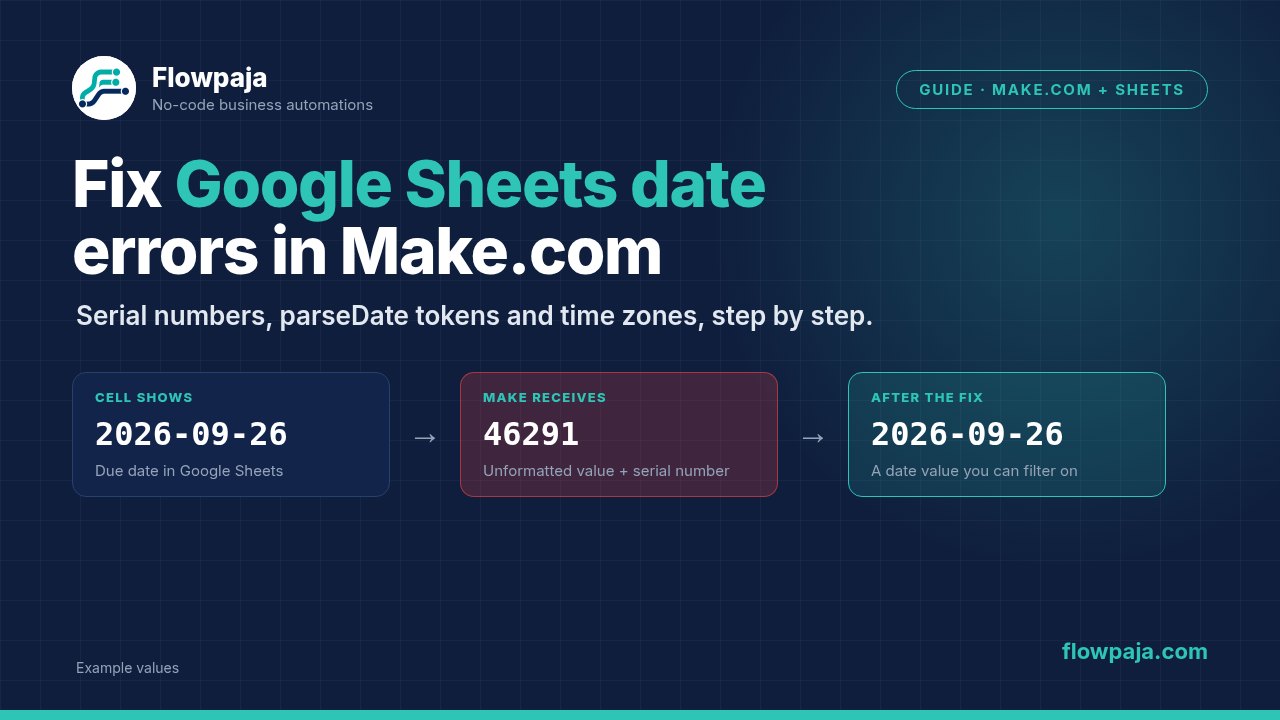
Your invoice sheet shows an ordinary due date. Make receives 46291, parseDate() fails, or your overdue filter lets the wrong invoice through. The row looks fine in Sheets, so the first thing to check is what Google Sheets actually sent to Make.
A date shown in a cell, a piece of text that looks like a date, and a date value inside Make are three different things. This guide builds a small test scenario with Google Sheets → Search Rows and two Tools → Set variable modules. You look at the raw value, parse it, check the result and then test an overdue filter. Use a separate test scenario and fictional invoices, not your live reminder scenario.
What Make can receive from a date cell
The same due date can reach Make in three forms:
2026-09-26: text. Parse it with the patternYYYY-MM-DD.26/09/2026: text. Parse it with the patternDD/MM/YYYY.46291: a Google Sheets date serial number. Change the module's render options, or convert the number (see the section on serial numbers below).
Google Sheets stores dates as numbers. The whole number counts the days since 30 December 1899, and the decimal part is the time of day as a fraction of a day. 46291 is 26 September 2026.
Which form you get depends on two settings in the Google Sheets Search Rows module (the Get a Cell and Get Range Values modules have the same two):
- Value render option. Formatted value returns what the cell shows, formatted with the cell's format and the spreadsheet's locale. Unformatted value returns the calculated value without formatting. Formula returns the formulas themselves.
- Date and time render option. Serial number returns dates as numbers such as
46291. Formatted string returns them as text in the cell's date format.
Google's Sheets API reference says the date and time option is ignored when the value option is Formatted value. So Unformatted value plus Serial number gives you 46291, and Formatted value gives you the date text you see in the cell.
In Make, parseDate() turns text into a date value and formatDate() turns a date value into text. Neither one reads a Sheets serial number directly. Make's date and time functions page lists both.
Step 1: Prepare a small test sheet
Create a tab named Date test with three headers: A: Invoice ID, B: Due date and C: Status.
Add four fictional invoices: one due yesterday, one due today, one due tomorrow and one with an empty due date. Set Status to Unpaid on all four. You don't need client names or email addresses for this test.
Open File → Settings and look at Locale and Time zone under General. The locale sets the spreadsheet's default date, number and currency formats, and a change applies to everyone who uses the file. Don't change it casually in a shared production sheet.
Select B2:B5 and choose Format → Number → Custom date and time. Arrange a four-digit year, two-digit month and two-digit day with hyphens between them. The cells should now read like 2026-09-26.
If the format changes nothing, the cell probably holds text. In a spare cell, =ISNUMBER(B2) returns FALSE for text and TRUE for a number. TRUE only tells you it's a number, so still check that it's the right date.
To turn a text date into a real date, =DATEVALUE(B2) works for date formats that Sheets would recognise if you typed them into a cell, and which formats those are depends on the spreadsheet's locale. It returns #VALUE! if B2 already holds a number, and it gives a plain number until you format the cell as a date. A date that Sheets has already read with day and month swapped can't be repaired with formatting. Type it again in the right order.
Step 2: See what Make actually receives
Create a new scenario and add Google Sheets → Search Rows. Set:
- Your Google connection and the test spreadsheet.
- Sheet Name:
Date test. - Table contains headers: Yes.
- Column range: a range that covers columns A to C.
- Filter: Status equal to
Unpaid. - Limit:
10, which is plenty for four rows. - Value render option: Formatted value.
If you can't see the render options, switch on the module's Advanced settings toggle.
Click Run once, open the module's output and find Due date. With the format from Step 1 it should read 2026-09-26. Write down the exact value before you change any formula, so you're fixing what Make received and not what the sheet seems to contain.
Step 3: Stop empty dates, then parse
Click the line after Search Rows to add a filter. Name it Has due date, choose the Due date item and the operator Exists. Make describes Exists as a check that the item is filled in, so the row with no due date stops here and never reaches parseDate().
After the filter, add Tools → Set variable. Set Variable name to parsed_due and Variable value to:
parseDate(1.`1`; "YYYY-MM-DD"; "Europe/Berlin")The first argument is the Due date item from Search Rows. In text form Make writes it as module 1, column 1, which is column B because Make counts columns from 0. Don't type it. Click Due date in the mapping panel and Make inserts the right reference for your scenario.
The third argument is the time zone. Europe/Berlin is only an example; use your business time zone's name from the tz database list, such as Europe/London or America/New_York, and use the same one in every formula in this guide. If you leave the time zone out, Make uses your organization's time zone. You'll find it under Profile → Time zone options, and only organization owners and admins can change it.
If your cells show 26/09/2026, use DD/MM/YYYY instead. The pattern has to match the incoming text exactly, separators included. Make lists every token in its date and time parsing tokens page.
Step 4: Check the parsed date
Add a second Tools → Set variable after the first one. Name it date_preview and set its value to:
formatDate(2.parsed_due; "YYYY-MM-DD"; "Europe/Berlin")Replace 2.parsed_due with the parsed_due item from your first Set variable module.
Click Run once and compare each preview with the sheet. The three rows with a due date should reach this module and the empty one should stop at the filter. Test with a day above 12, such as 26 September: a value like 09/10/2026 looks plausible even when September and October have been swapped.
Don't judge the result by the raw parsed_due value in the output. Make shows dates in module output in your user time zone (the Web entry under Profile → Time zone options), which only changes the display. If that zone differs from the one in your formula, parsed_due can show a different hour or even a different day. The date_preview text is the reliable check.
Step 5: Test the overdue boundary
When the previews are right, add a second filter on the line between the two Set variable modules. Name it Overdue. Here, overdue means a due date before today in your business time zone.
- First field: the parsed_due item from module 2.
- Operator: Datetime operators: Earlier than.
- Second field:
parseDate(formatDate(now; "YYYY-MM-DD"; "Europe/Berlin"); "YYYY-MM-DD"; "Europe/Berlin")This gives you midnight at the start of today in that time zone. If you compare with now instead, an invoice due today also passes, because midnight this morning is earlier than the current time.
Datetime operators only work properly when both sides are date values. Text from formatDate() won't compare correctly. If every row passes the filter, put the parseDate() expression from Step 3 straight into the first field instead of the variable.
Run the test again. You should see:
- Due yesterday: reaches date_preview.
- Due today: stops at the Overdue filter.
- Due tomorrow: stops at the Overdue filter.
- Empty due date: stops at the Has due date filter.
Only copy the date logic into your real reminder scenario once these results match. Keep that scenario's status checks, reminder timing and duplicate protection. A correct date filter on its own doesn't decide who should get an email.
If you need to keep serial numbers
Formatted value is the simpler route. If another scenario needs the Unformatted value setting and you get whole-number serials, convert them explicitly:
formatDate(addDays(parseDate("1899-12-30"; "YYYY-MM-DD"; "UTC"); 46291); "YYYY-MM-DD"; "UTC")This returns the text 2026-09-26. Replace 46291 with your mapped Due date item. To compare the result with other dates, parse that text in your business time zone as in Step 3.
This only works for whole days. A serial with a decimal part also carries a time of day, and the number doesn't say which time zone that time was in, so don't reuse this formula for appointments or timestamps without working that out first.
Common errors
The pattern doesn't match the input. 26/09/2026 needs slashes in its pattern; YYYY-MM-DD describes a different string. Check the output again after you change a cell format.
Month, minute and weekday tokens are mixed up. In Make, MM is the month and mm is minutes. DD is the day of the month, while dd is a short weekday name. Case matters, and Make's tokens differ from the ones in Google Sheets' own custom formats, so use Make's date and time formatting tokens page.
The preview shows the previous day. Look at the time zones. Midnight in one zone can be the previous day in another. Use the same time zone in parseDate() and formatDate(), and remember that leaving it out means your organization's time zone.
The Exists filter passes but parsing fails. Text such as TBD isn't empty. Fix it in the sheet. Don't replace missing or invalid due dates with today's date.
Make still receives 46291 after you changed the cell format. The module is set to Unformatted value with Serial number. Switch Value render option to Formatted value, or convert the number as shown above.
Amounts changed after you switched to Formatted value. The setting applies to every column, not just dates. A currency cell that used to arrive as 1.23 can arrive as $1.23. Check the mappings that use amounts before you move the change to a live scenario.
Use it in an invoice reminder scenario
For the full build, see our invoice payment reminders guide. If you only want late invoices flagged inside the sheet, with no Make at all, see how to highlight overdue invoices in Google Sheets. For errors that aren't about dates, such as expired connections or rate limits, see 10 common Make.com scenario errors.