How to Highlight Overdue Invoices in Google Sheets (Formulas + Conditional Formatting)

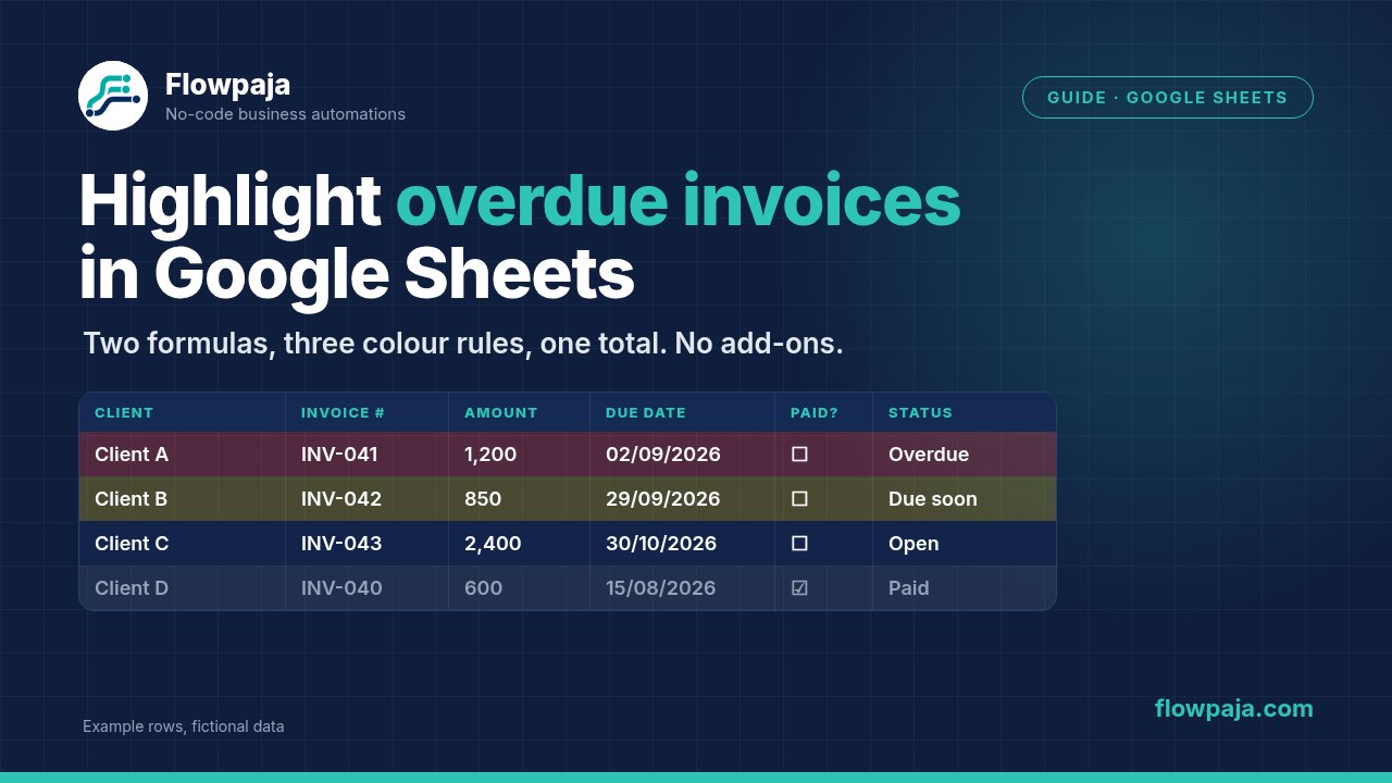
If you track invoices in a spreadsheet, you've probably scrolled through it trying to work out which clients are late. Google Sheets can do that for you. It can count how many days each invoice is overdue, label every row, colour the late ones red, and total how much money you're waiting on.

This guide builds that tracker step by step. Every formula is in a code block with a plain-English explanation, so you can copy it and understand what it does.

The Invoice Tracker Layout

Create a sheet (tab) called Invoices with these headers in row 1:

• A: Client, the client name
• B: Invoice #, e.g. INV-042
• C: Amount, a plain number, e.g. 1200
• D: Due Date, a real date, e.g. 15/10/2026
• E: Paid?, a checkbox
• F: Days Overdue, a formula
• G: Status, a formula

Two setup tips:

• Paid? column: select E2:E500 and choose Insert → Checkbox. A ticked box counts as TRUE and an unticked one as FALSE, which makes the formulas simpler.
• Due Date column: select D2:D500 and choose Format → Number → Date, so the entries display as dates. Formatting doesn't convert text that only looks like a date, though (see Common Mistakes).

Your data starts in row 2. The formulas below go in row 2, and you copy them down: drag the small square at the bottom-right of the cell, or double-click it.

Formula 1: Days Overdue

The basic version

Put this in F2:

=IF(OR(D2="", E2=TRUE), "", MAX(0, TODAY()-D2))

In plain English:

• TODAY() returns today's date. It updates automatically.
• TODAY()-D2 subtracts the due date from today. Sheets stores dates as numbers, so the result is a number of days.
• MAX(0, …) shows 0 instead of a negative number when the invoice isn't due yet.
• IF(OR(D2="", E2=TRUE), "", …) leaves the cell blank if there's no due date or the invoice is already paid. Without this check, an empty due date is treated as a date back in 1899 and shows a huge number.

A safer version that catches text dates

If dates are sometimes pasted in from emails or other tools, some of them may be stored as text, which Sheets can't calculate with. This version flags them:

=IF(OR(D2="", E2=TRUE), "", IF(ISNUMBER(D2), MAX(0, TODAY()-D2), "Check date"))

In plain English: a real date is stored as a number, so ISNUMBER(D2) is TRUE for real dates and FALSE for text that only looks like a date. Text dates show "Check date" instead of a wrong result or an error.

Formula 2: Status (Paid / Due soon / Overdue)

Put this in G2:

=IF(A2="", "", IF(E2=TRUE, "Paid", IF(D2="", "No due date", IF(NOT(ISNUMBER(D2)), "Check date", IF(D2<TODAY(), "Overdue", IF(D2-TODAY()<=7, "Due soon", "Open"))))))

In plain English: Sheets checks the conditions in order and stops at the first one that's true.

1. No client name means an empty row, so the cell stays blank.
2. The Paid? box is ticked: Paid.
3. No due date: No due date, so you notice the missing information.
4. The due date is text, not a real date: Check date. Without this check, a text date would show an error here.
5. The due date is before today: Overdue.
6. The due date is today or within the next 7 days: Due soon.
7. Anything else: Open.

To change the "due soon" window, replace 7 with another number of days.

Conditional Formatting: Colour Whole Rows

Now make overdue rows red, rows due soon yellow, and paid rows grey.

How to add a rule

1. Select A2:G500, starting from row 2, not the header row.
2. Go to Format → Conditional formatting.
3. Under "Format rules", open the "Format cells if…" dropdown and choose Custom formula is.
4. Paste the formula, pick a fill colour, and click Done.
5. Use Add another rule for the next one.

Rule 1: Overdue (red)

=AND(NOT($E2), $D2<>"", $D2<TODAY())

In plain English: colour the row if the invoice is not paid, has a due date, and that date is before today.

Rule 2: Due soon (yellow)

=AND(NOT($E2), $D2<>"", $D2>=TODAY(), $D2-TODAY()<=7)

In plain English: the invoice is unpaid and due today or within the next 7 days.

Rule 3: Paid (grey)

=$E2=TRUE

In plain English: the Paid? box is ticked. Grey text or a light grey fill works well, so paid invoices fade into the background.

A simpler option: use the Status column

Your Status column already does the logic, so you can base the colours on it instead:

=$G2="Overdue"

This is easier to maintain, because you only change the logic in one place. The trade-off is that the colours depend on the Status formula being filled down to every row.

Why the dollar signs matter

$E2 means "always column E, but the row changes." Sheets applies the formula to each cell in the range, working out the row relative to row 2. The $ locks the column, so every cell in a row, from A to G, checks that row's Paid? and Due Date cells. Without it, cell B2 would check F2, cell C2 would check G2, and so on, and your colouring would look random.

Total Overdue Amount (SUMIFS)

Put this in a summary cell, for example L2, with a label like "Total overdue" in K2. That keeps columns H to J free in case you add columns later:

=SUMIFS(C2:C, G2:G, "Overdue")

In plain English: add up the amounts in column C for every row where column G says "Overdue". C2:C means "from C2 to the bottom of the column", so new invoices are included automatically.

If you'd rather not depend on the Status column, calculate it from the raw data:

=SUMIFS(C2:C, D2:D, "<"&TODAY(), E2:E, FALSE)

In plain English: add up the amounts where the due date is before today and the Paid? box is unticked. The "<"&TODAY() part combines the "less than" sign with today's date to build the condition. This version only counts rows that have a checkbox, because an empty cell isn't the same as FALSE.

To count the overdue invoices instead of totalling them:

=COUNTIF(G2:G, "Overdue")

A View of Only Overdue Invoices (FILTER)

Create a second tab called Overdue and put this in A2, with the same headers as the Invoices tab in row 1:

=IFERROR(SORT(FILTER(Invoices!A2:G, Invoices!G2:G="Overdue"), 4, TRUE), "No overdue invoices")

In plain English:

• FILTER(Invoices!A2:G, Invoices!G2:G="Overdue") returns every row from the Invoices tab whose status is Overdue.
• SORT(…, 4, TRUE) sorts those rows by the 4th column (Due Date), oldest first, so the most overdue invoice is at the top.
• IFERROR(…, "No overdue invoices") handles the case where nothing is overdue. Otherwise FILTER shows an error.

The view updates by itself. Don't type anything below or to the right of A2 on that tab (columns A to G), because the formula needs that space to show its results. If something is in the way, you'll see a #REF! error instead. If the due dates show up as plain numbers, format column D on this tab with Format → Number → Date.

Common Mistakes

Dates stored as text

Symptom: Days Overdue or Status shows "Check date" (or the basic Days Overdue formula shows #VALUE!), or the conditional formatting ignores some rows.

Why: The date was typed or pasted in a format your spreadsheet's locale doesn't recognise, for example 10/15/2026 in a sheet set to a day/month locale, or it went into a cell formatted as Plain text. Sheets then stores it as text. Text dates usually line up on the left of the cell, and real dates on the right.

Fix: Check your locale under File → Settings. The simplest fix is to re-enter the date in the format that locale expects. For many rows, use a helper column. If the text is in a format your locale does recognise (typical for Plain text cells), this converts it:

=DATEVALUE(D2)

DATEVALUE only understands the same formats Sheets recognises when you type a date, so it fails on 10/15/2026 in a day/month sheet. For text in month/day/year order, build the date from its parts instead:

=DATE(INDEX(SPLIT(D2, "/"), 1, 3), INDEX(SPLIT(D2, "/"), 1, 1), INDEX(SPLIT(D2, "/"), 1, 2))

Then paste the result back as values (Edit → Paste special → Values only) and format it as a date.

Comma vs semicolon separators

Symptom: You paste a formula and get a parse error.

Why: In many locales that use a comma as the decimal separator (a lot of European ones, for example), Sheets uses semicolons between function arguments. This guide uses commas.

Fix: Replace the commas between arguments with semicolons:

=IF(OR(D2=""; E2=TRUE); ""; MAX(0; TODAY()-D2))

Don't change commas that appear inside quoted text.

Wrong or missing absolute references

Symptom: Only one column turns red, or the colours are shifted one row up or down.

Why: The formula is missing $ before the column letter, or its row number doesn't match the first row of the "Apply to range" box. If the range starts at A2, the formula must refer to row 2, e.g. $D2. If it starts at A1, it must use $D1.

Fix: Make the range start and the formula's row number match, and put $ before the column letters.

Amounts stored as text

Symptom: The SUMIFS total is 0 or too low.

Why: Amounts typed as "€1.200,00" or "1200 EUR" may be stored as text.

Fix: Type plain numbers and use Format → Number → Currency to display the symbol.

Rules in the wrong order

Symptom: A paid invoice still shows red.

Why: When several rules match a cell, the one higher in the list wins. Sheets doesn't combine them.

Fix: In the conditional formatting panel, drag the rules into the order you want. The red and yellow rules above also include NOT($E2), so a ticked Paid? box keeps a row out of them whatever the order.

Wrapping Up

With two formulas, three colour rules, one total and one filtered view, your spreadsheet shows who owes you money as soon as you open it. Start with the Days Overdue and Status columns, add the colours, then add the total and the Overdue tab. If something looks wrong, it's almost always a text date, a separator mismatch, or a missing $.